Sheet metal processing lines: how to calculate productivity, availability and efficiency
Sheet metal production lines nowadays are more and more automated, with increasing number of processing modules. Knowing how to balance a production system has become a strategic skill for the production manager in order to optimize the line and increase the productivity.
Production systems consist of a series of machines, each one performing one part of the process. In sheet metal processing lines, for example, a system can include uncoiling, punching, laser cutting, forming, roll forming, welding and packaging.
To calculate the productivity and efficiency of a given production system, it is essential to understand the performance of each machine/module of the line, and how these modules are connected.
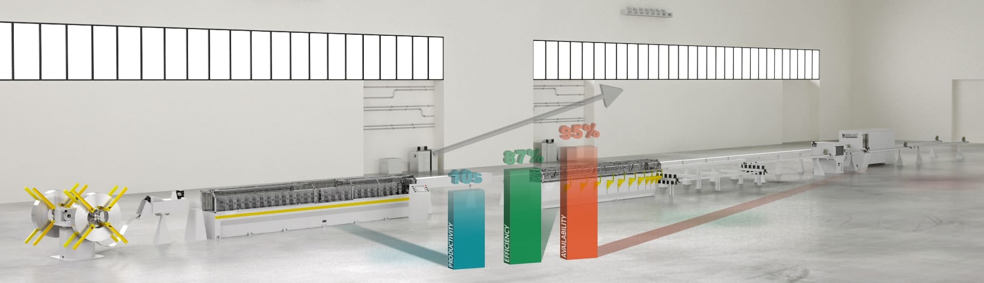
This guide illustrates a simple methodology to calculate productivity, availability and efficiency of complex production systems, given the main parameters of each module.
You can find more details related to these concepts into the book “The Revolution of Efficiency” that you can request here:
REQUEST THE BOOK FOR FREE
Defining the line and the processing modules
From now on I will define a line as a series of processing modules, each one characterized by the parameter “cycle time” or productivity P: expressed in seconds per part, is the amount of time the module is engaged to complete its process, including loading, processing and unloading time.
Another parameter that characterizes a module is the availability A, defined by this formula:
A = (Mean Time Between Failures)/((Mean Time Between Failures) + (Mean Time To Repair))
Each module is defined by the previous two parameters, and between each module we can have a buffer (parallel processing) or not (serial processing).
The previous parameter will be used to estimate, together with other considerations, the line efficiency E. Expressed as a percentage, this is the expected productivity over an extended period of time, including the preventive maintenance and setup time. For example, a line with 85% efficiency means that it will be active in production 85% of the time.
Calculating the Productivity of the line
When we know the Productivity of each module, we can calculate the Productivity of the line in three different cases.
Simultaneous processing
In the first case, the modules have buffers inbetween, so each module carries on its operation on simultaneously on different parts down the line stream.
The Productivity P will be in this case the maximum value of the Productivities P of each module. This module is the bottleneck of the system.
P = MAX (P1, P2, P3…, Pn)
For example, in a processing line for venetian blinds, we identify three modules:
- Roll forming and punching, P1 = 10 seconds per part
- Module for head pin positioning, P2 = 5 seconds
- Module for hooks insertion and loop tape assembly, P3 = 8 second
The Productivity of the complete line will be, in this case 10 seconds per part.
The following video shows one line for venetian blinds in operation.
A third example of line with simultaneous processing is the coil punching and simultaneous laser cutting line.
Here, the punching and laser operation are separated by a roller table that acts as a buffer and the punching and laser operation take place simultaneously.
For example in the processing of the part we identify two modules:
- Decoiling and punching, P4 = 25 seconds
- Laser cutting, P5 = 33 seconds
The productivity of the line will be, in this case, 33 seconds.
The following video explains in detail the function of the punching and simultaneous laser cutting lines.
Serial processing
In the second case, the modules are tightly connected and work without a buffer, i.e. in serial processing.
The productivity P will be in this case the sum of the Productivities P of each module.
P = P1 + P2 + P3 + … + Pn
Some lower productivity lines for venetian blinds have this kind of operation.
With the same example of the previous venetian blind line, the productivity becomes:
P = P1 + P2 + P3 = 10s + 5s + 8s = 23 seconds – a 130% increase in the cycle time.
Also coil fed punch laser combo are can be built with the two modules attached, working in serial configuration as you can see in the following video.
The productivity in this case is:
P = P4 + P5 = 25s + 33s = 58 seconds – a 75% increase in the cycle time.
It is clear that adding buffers can lead to a significant increase of the productivity, and of the availability of the system as well. In large plants, the buffers can be very large and if one of the modules has a function problem, they sometimes have the possibility to divert the production flow to a second backup module.
Serial + Simultaneous processing
In the third case, some modules are positioned in simultaneous processing and others in serial processing. In this case, the serial modules will be seen as a new module with Productivity P equal to the sum of the two productivities.
For example, if the line has:
- A first module with performance P6 = 8 seconds, followed by a buffer
- The following modules with P7 = 7 seconds and P8 = 12 seconds positioned in serial processing configuration.
The productivity of the line will result in:
P = MAX (P6, (P7+P8)) = MAX (8s, (7s + 12s)
P = MAX (8s, 19s) = 19 seconds
Calculating the Availability
Each module, as any machine, is characterized by an availability that can be expressed in percentage. Availability is defined as:
A = (Mean Time Between Failures)/((Mean Time Between Failures) + (Mean Time To Repair))
Also written as:
A = MTBF / (MTBF + MTTR)
In production lines, the availability of each module has a direct influence on the availability of the complete line. A conservative calculation for the line availability is the following.
A = A1 * A2 * A3 * … * An
Consider three modules with different availabilities:
- A1 = 99% = 0,99
- A2 = 99,9% = 0,999
- A3 = 98,5% = 0,985
A = 0,99 * 0,999 * 0,985 = 0,974 = 97,4%
I consider that the same calculation is valid for serial or simultaneous configuration, since a malfunction in one of the modules, stops the complete line in both cases.
Defining the Efficiency
The calculated productivity indicates the cycle time per part in continuous production. The line, however, can be non productive for a number of reasons:
- raw material change – for example a coil change
- change of tooling or configuration – for example at the end of one production batch
- for preventive maintenance
These times depend on the machine design, of course, but also on the organization of the production, number of material changes per week or day (for example in case of frequent color changes) and on the technicians’ skills.
I call these times as Setup Times or ST and they have to be either measured or estimated. Since efficiency is defined as expected productivity over an extended period of time, I suggest estimating the ST value in the production of a large enough batch of N parts – for example the quantity that is expected to be produced in one week.
Efficiency E can be calculated conservatively as follows:
E = N * P / (N * P + ST) * A
I use the availability value to take into account any stop caused by the modules.
For example, if we have:
- N = 10000 parts
- P = 12 seconds per part
- ST = 7 hours
- A = 97,4%
E = 120000 / (120000 + 25200) * 0,974 = 0,805 = 80,5%
The production manager can use this Efficiency value – knowing it is an estimation – to calculate the line Gross Productivity GP and simplify his calculations.
GP = P / E
In the previous example, with P = 12 seconds and E = 80,5%:
GP = 12 / 0,805 = 14,9 seconds per part
This means that, even if the machine produces one part every 12 seconds, we have to consider 14,9 seconds to take into account the setup times and the availability of the system.
In one week, with 144000 seconds totally available, the line will be able to produce:
N = 144000s / 14,9s = 9660 parts
Notes
The calculations have been presented in a conservative way, but two additional factors should be considered.
- If the machine or system relies to an operator feeding or discharging the line, the productivity will have to consider the efficiency of the operator.
- We assumed the line producing 100% good parts: if the line is less efficient, the percentage of scrap will reduce the calculated efficiency of the line.
Conclusions
The formulas I proposed, represent a simple methodology that can be applied to a number of sheet metal working systems: punching machines, laser cutting systems, FMS, roll forming machines and packaging systems.
In the article I pointed out how the Efficiency depends also on the manufacturer’s organization. In fact, larger batches reduce the impact of Setup Times ST in the calculation. However, in today’s competitive markets, sheet metal manufacturers need to be able to react quickly to customers’ requests: this turns out in smaller batches, increased setup time and reduced efficiency.
Even in this case, improving the efficiency is possible with a careful organization of the production and, of course, with the use of modern and flexible lines with lower setup times.
Author
Andrea Dallan – C.E.O. of Dallan Spa